How much of a Gated DeltaNet state is actually in use, and what happens when you throw the rest away.
Every linear-attention head in Qwen3.5-0.8B carries a 128×128 matrix as its memory. After 16K tokens of context, the numerical rank of that matrix is 127 in most heads. It looks full. Measured properly, no head in the model uses more than about 44 directions, the median head uses 8, and a quarter use fewer than 3. This post is about what “uses” means there, why the number comes out where it does, and whether the apparently empty part of the matrix does anything. The short version: for perplexity it does nothing; for retrieval it does more than perplexity can see; and for one task it is actively in the way.
Everything below is measured on the unmodified Qwen3.5-0.8B backbone (18 Gated DeltaNet layers, 6 full attention layers, 16 heads of 128×128 per linear layer) unless a distilled control checkpoint of the same architecture is named.
1. Rank, measured honestly
Numerical rank counts singular values above the float32 floor. In a decaying recurrence that is the wrong question: a direction written 15K tokens ago has been multiplied by $\alpha$ thousands of times, but it is still above $\sigma_{\max} \cdot 128 \cdot \varepsilon$ and still counts. Almost every head therefore reports rank 126 or 127.
Effective rank asks how many directions carry the norm. With singular values $\sigma_{i}$ and
$$p_{i} = \frac{\sigma_{i}}{\sum_{j} \sigma_{j}},$$
the effective rank is
$$\operatorname{erank} = \exp\left(-\sum_{i} p_{i} \log p_{i}\right):$$
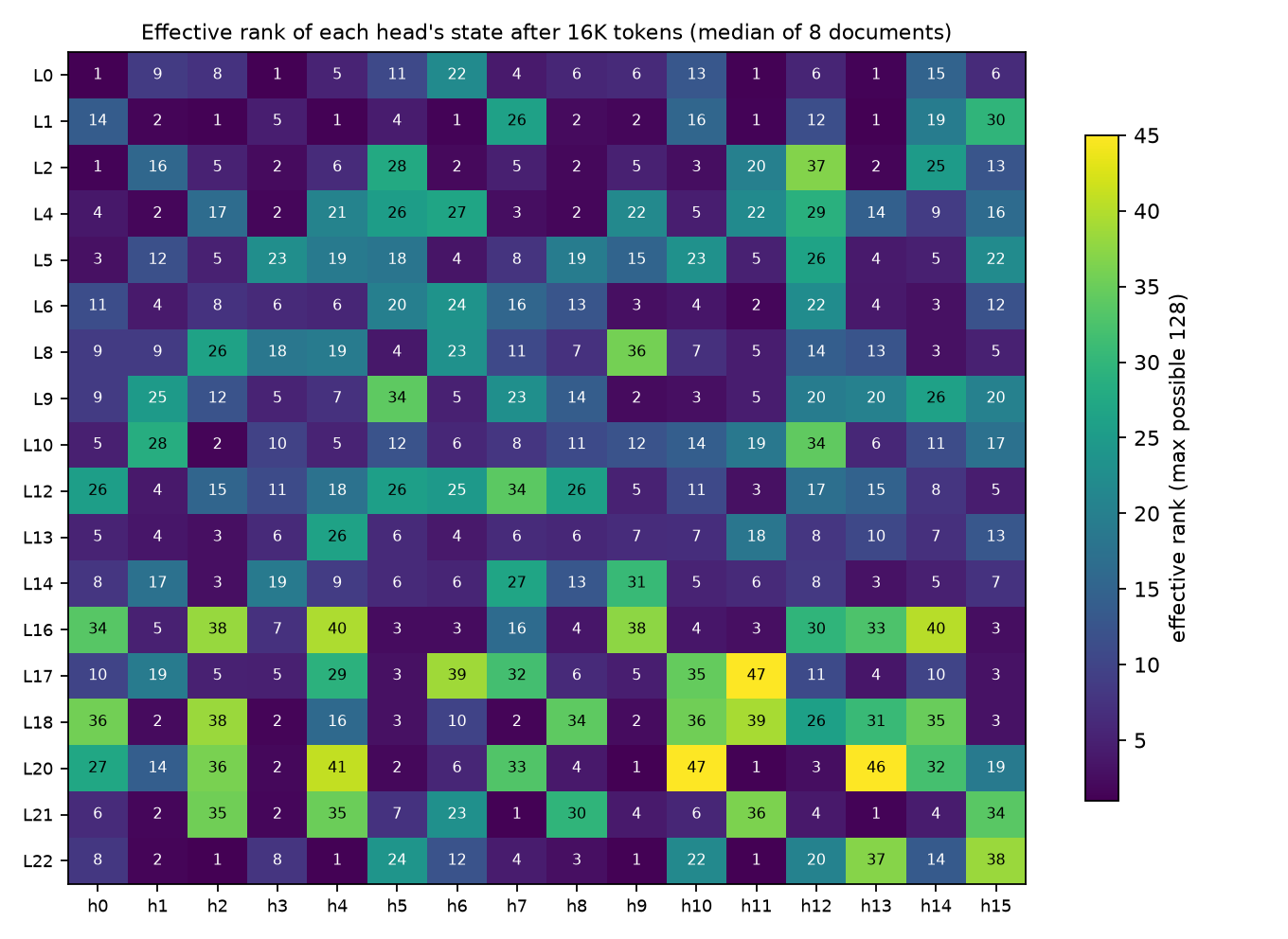
128 for a flat spectrum, 1 for a single outer product. Computed on the carried state of every head after 16,384 tokens of a single document, median over eight documents:
| statistic over 288 heads | value |
|---|---|
| maximum effective rank | 43.5 |
| median | 8.2 |
| heads at or below 3 | 19% |
| heads below 10 | 53% |
| heads above 25 | 19% |
The min–max spread across the eight documents is tight for nearly every head, so this is a property of the head, not of the text it happened to read. The heads with numerical rank 127 have effective ranks of 30 to 44 at best, and in layer 0 some of them sit at 5 to 8: numerical rank 127 was decayed residue.
2. What sets the number
The obvious hypothesis is the decay horizon. A head with per-token decay $\alpha$ forgets in about $\frac{1}{1-\alpha}$ tokens, and repeated writes to the same key converge under the delta rule rather than piling up, so the state should hold roughly as many directions as there are distinct keys inside the horizon. That is the right first-order story: across heads, effective rank against horizon has Spearman correlation 0.91.
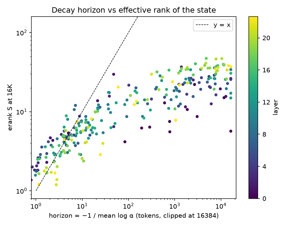
But the points do not follow y = x. Heads with horizons under 10 tokens sit on the diagonal; heads with horizons of 5,000 to 10,000 tokens plateau at 30 to 47. Something other than decay caps them, and it is the keys. For those heads the L2-normalised keys live in a narrow cone: the mean key has norm 0.8 to 0.94, and the plain covariance of the keys written inside the horizon has an effective rank of only 3 to 6. The state reaches rank 40 at all only because the delta rule cancels the shared component of every key and lets the small residuals accumulate. Key diversity, not decay, is the ceiling.
Two consequences follow. Sixty-one percent of heads forget within 256 tokens, so most of the recurrent state is a short-range mixer whatever its rank. And the long-horizon heads are not full: they have the horizon to hold thousands of tokens of content and the key geometry to hold a few dozen directions of it.
(A footnote on a tempting comparison: the decayed key covariance $P$ of those long heads has an effective rank of 2 to 6, far below the state’s 35 to 47. That is not a contradiction. Eigenvalues of a covariance are squared amplitudes and singular values of the state are not; on the same scale the two agree.)
3. Does the rank matter?
Effective rank says where the norm is. It does not say whether the model reads anything from the faint directions. The way to find out is to remove them and watch the model.
The intervention. Run the model in 256-token segments through its cache. At every segment boundary, take each head’s carried state, compute its top $r$ left singular directions, and replace the state by its projection onto them. The truncated state is what the next segment reads and what it writes into, so the cut compounds: the model keeps at most $r$ directions of memory older than one segment, plus whatever the current segment adds. $r = 128$ is the untouched model. The truncation is applied to every head of every linear layer at once; the six full-attention layers are never touched.
Making it cheap. An exact batched SVD of the 288 head states costs about 1.7 s per boundary on an L20X, which is 64 boundaries per 16K prompt. Subspace iteration on $SS^{\top}$ in float64 with Cholesky-QR and a $q \times q$ Rayleigh–Ritz step ($q \le 32$, so the small eigenproblem stays on cuSOLVER’s batched Jacobi path) gives the same truncation to within $10^{-5}$ of retained energy in about 10 ms. The whole probe is a few hundred lines on top of
flash-linear-attentionand runs on any model whose cache exposes the state.
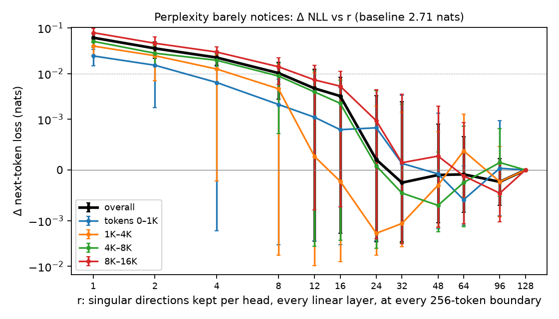
Perplexity says the residue is dead. Mean next-token loss over the same eight documents, as a function of $r$, with the difference to the untouched model:
| r kept per head | Δ NLL (nats) |
|---|---|
| 48 | −0.0001 ± 0.0010 |
| 24 | +0.0002 ± 0.0031 |
| 12 | +0.0047 |
| 4 | +0.0224 |
| 1 | +0.0611 |
Nothing above the effective rank is read. Keeping 12 directions per head costs half a percent of the loss; keeping one direction costs 2%. Tokens whose preceding bigram already appeared more than 512 tokens earlier, the copy-and-induction cases, are no more sensitive than the average token. On web text, the far memory of the entire recurrent stack is worth 0.06 nats, and the full-attention layers are doing the copying.
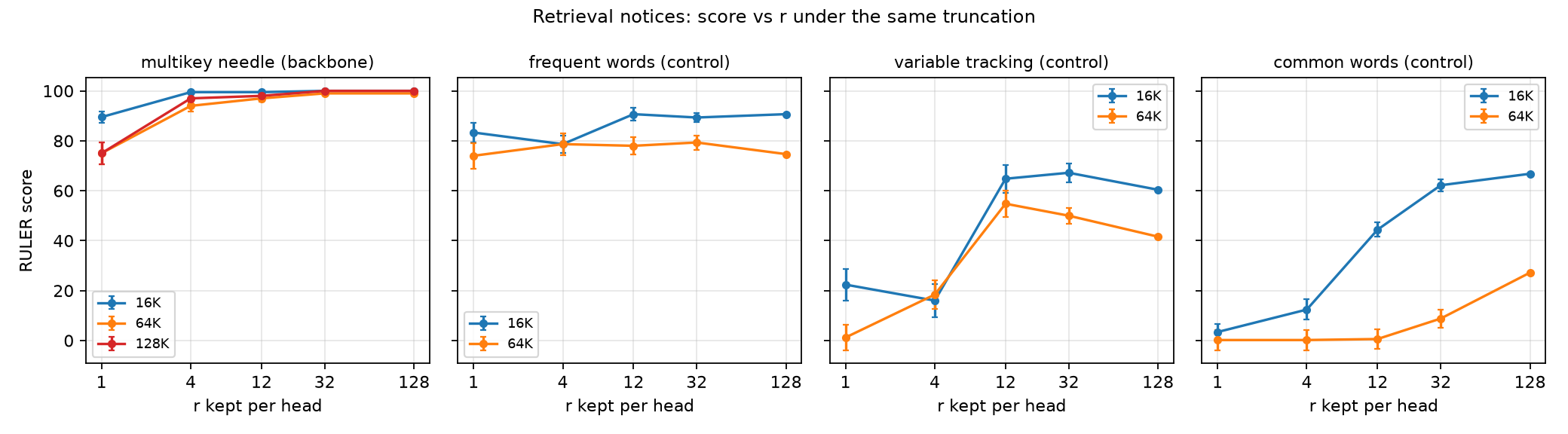
Retrieval says otherwise. The same truncation, but the prompt is a RULER task and the metric is whether the model answers. Scores are RULER’s string match on 50 to 200 samples; the distilled control checkpoint is used for the aggregation tasks because the base model’s prompt handling on them is fragile.
| r kept per head | multikey needle, 64K | frequent words, 64K | variable tracking, 16K | common words, 16K |
|---|---|---|---|---|
| 128 | 99 | 75 | 60 | 67 |
| 32 | 99 | 79 | 67 | 62 |
| 12 | 97 | 78 | 65 | 44 |
| 4 | 94 | 79 | 16 | 12 |
| 1 | 75 | 74 | 22 | 3 |
The rank-1 model that lost 2% of perplexity loses a quarter of the needles at 64K and 128K and almost all of variable tracking. Perplexity on web text simply cannot see long-range state usage, because nothing in a web document depends on a specific fact from thousands of tokens back.
The working rank is small but it depends on the task. Single-needle retrieval survives with about 4 directions per head. Picking the three most frequent words out of 64K tokens needs one direction, which is what an exponential moving average of values is. Tracking chains of variable reassignments needs about 12 and collapses at 4. Counting the ten most common words in a 16K list is the first workload that wants more: 12 directions cost 22 points and 32 still cost 5. At 64K the same task loses 18 of its 27 points already at $r = 32$. That is the one place in these measurements where the size of the state is the binding constraint, and it is a many-item aggregation, not retrieval.
One more thing the table shows. For variable tracking at 64K, keeping only the top 12 to 32 directions improves the score by 8 to 19 points, on both the backbone and the control, with paired standard errors of 3 to 5. The faint tail of the state, the decayed content that effective rank ignores, is not memory for this task. It is interference.
4. What to take from it
- Effective rank is a horizon-and-key-diversity measurement, not a content measurement. It tells you how long a head remembers and how correlated its keys are. It does not tell you what the head is storing, and in this model the long heads store a few dozen directions out of a possible 128 because their keys are nearly parallel.
- Web-text perplexity is blind to the recurrent memory. A model that has lost a quarter of its long-range retrieval reads as a 2% loss change. Any claim about state capacity needs a retrieval or aggregation metric.
- The working rank is 4 to 12 for most tasks and more than 32 for one. Most heads could run with a much smaller state and nothing measurable would change. The exception is many-item counting, which is also the task the model is worst at.
- The low-energy tail is noise for tracking tasks. Removing it helps. That argues for less cross-talk in the state, through shorter effective horizons or less correlated keys, and against readouts that amplify faint directions.
The caveats are the usual ones and they are real. This is one 0.8B model, a hybrid whose attention layers were left intact, so every number is “linear state on top of full attention”. Eight documents for the perplexity probe, fifty samples per aggregation cell, so differences under about five points are noise. The truncation runs every 256 tokens, so $r$ counts directions of carried memory and says nothing about what a head does within a segment. And the common-words baseline at 64K was already weak, so its collapse is consistent with a capacity limit rather than proof of one.
The open question is the interesting one. If common-words at 64K is rank-limited, some specific heads are carrying the count. Widening only those, and shrinking the sixty percent of heads that forget within a segment, would be a nearly free trade if the counting heads can be found. That is a per-layer, then per-head, version of the same truncation, and it is the next thing to run.